Statistics theory

Normal distribution written in exponential family form

Ancillary precision (how ancillary statistics helps when estimating $\theta$)

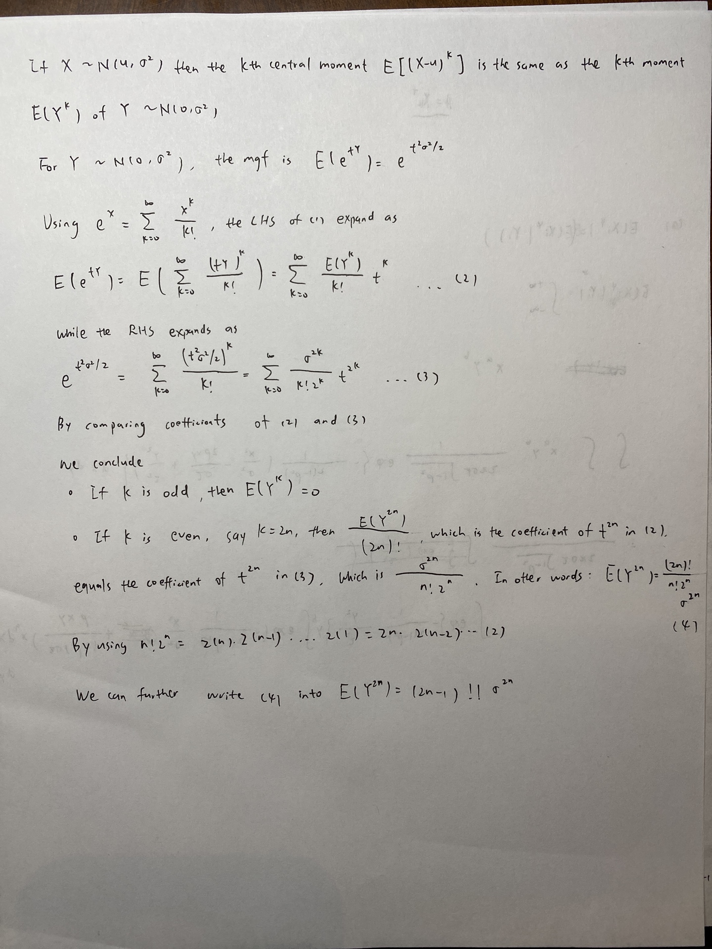
Moments of normal distribution

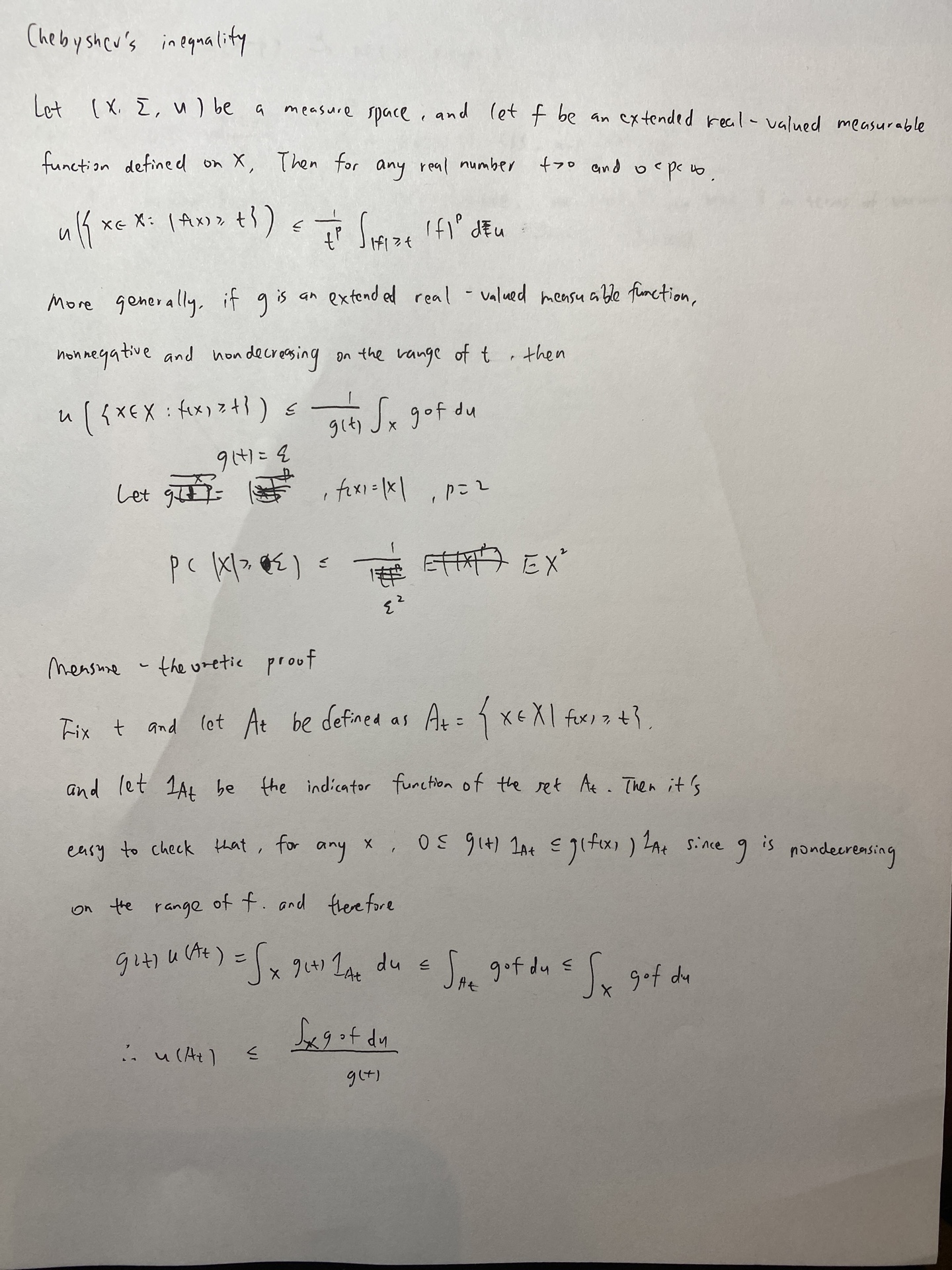
chebyshev’s inequality

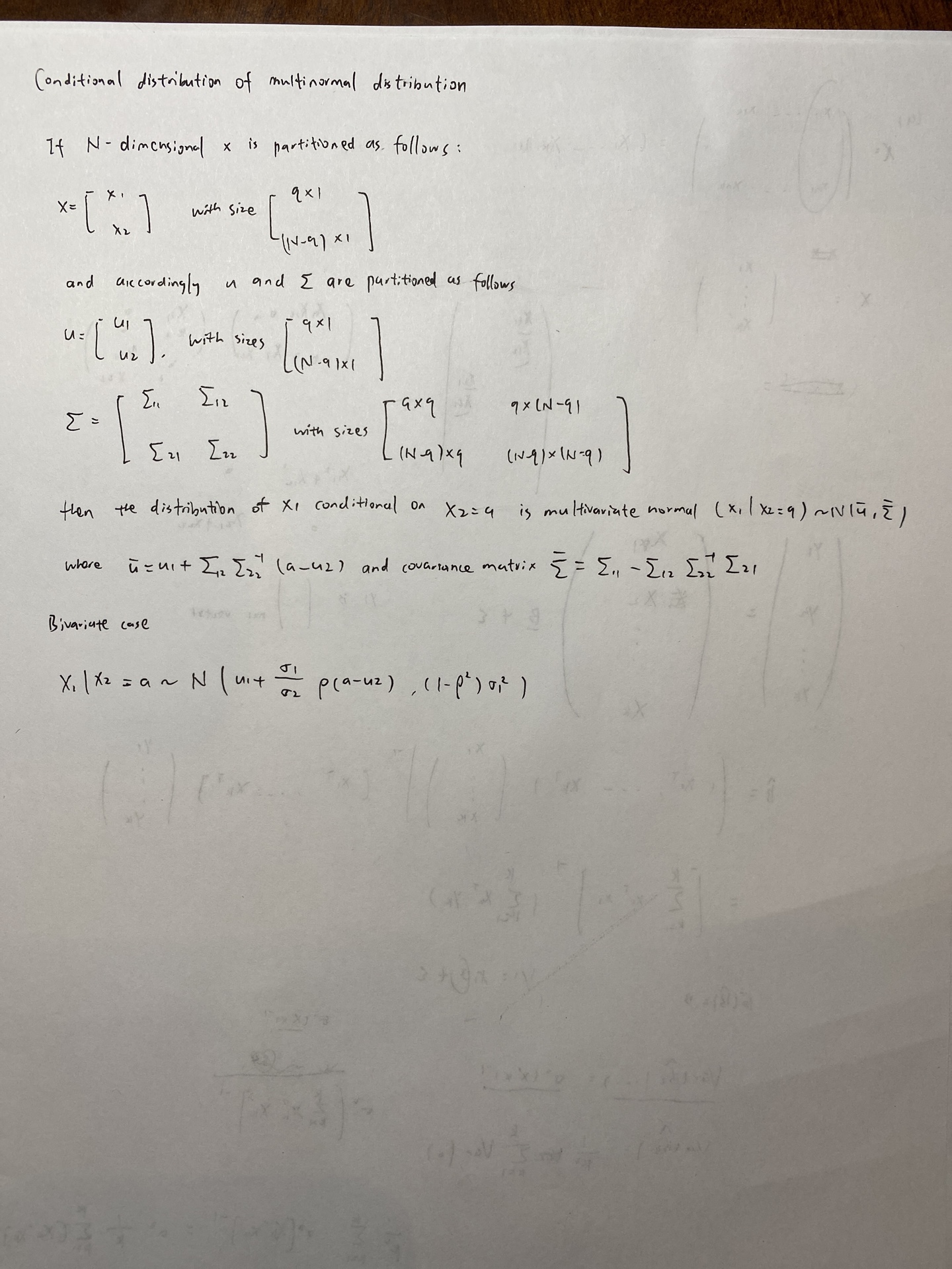
Conditional distribution of multinormal distribution

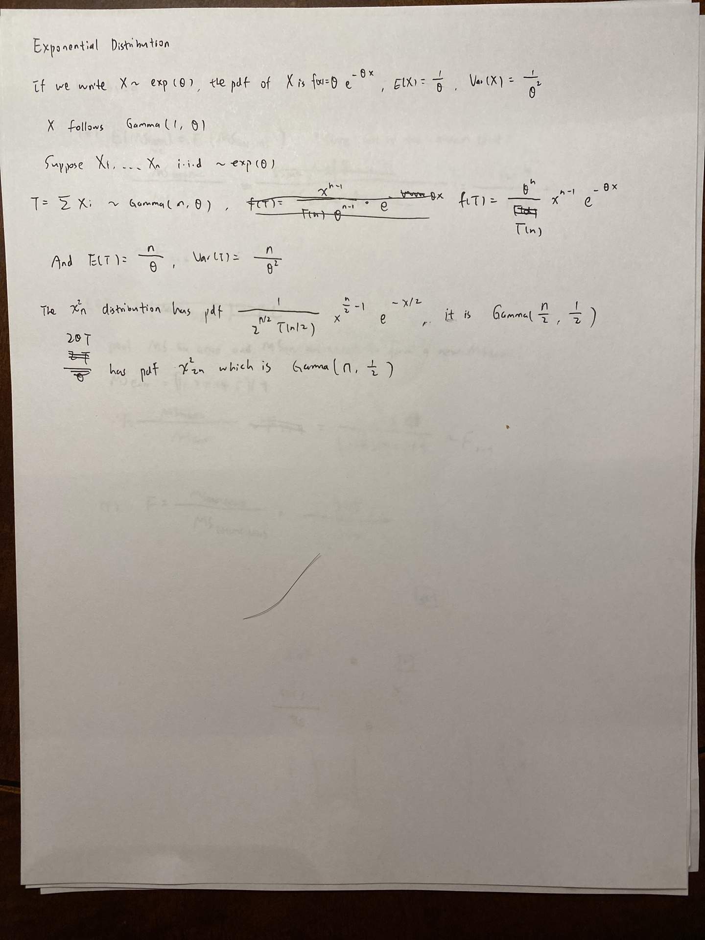
Exponential distribution, gamma distribution and chi-square distribution

Multiparameters MLE

If we have some restrictions on $\theta$, say $\theta > 0$ ，

MLE may not be unique

MLE in exponential family

Bayes estimator

Intuition: If $\theta$ is fixed, we want to find a estimator to estimate $\theta$ such that its mse is minimized. Since due to bayesian point of view, our goal becomes:

Proving the crammer rao lower bound

UMVUE in normal distribution

Situations that the key condition for crammer-rao lower bound is violated.

UMVUE is uncorrelated with all estimators which are unbiased to 0

An alternative to Theorem 7.3.20 is that

Example that UMVUE does not exist

Lehmann-Scheffe Theorem

FInd a complete statistics in uniform distribution

If we are estimating $g(\theta)$ instead of $\theta$,

To show this, intuitively, we can go back to

Here, we take derivative to $\theta>1$, we can only get the result that $g(t) = 0$ for all $t>1$.

there exsits many choices of $g(t)$ to make $g(t) \neq 0$ when $0<t<1$.

UMVUE in poisson family

Prove S is not unbiased for sigma

UMVUE in normal family

UMVUE is exponential distribution family

UMVUE in simple linear regression

UMP test using Neyman-Pearson lemma

Existence of UMP without monotone likelihood ratio

How to show the UMP test does not exist

UMPU test in exponential family

Definition of the p-value

Definition of confidence coefficient

Confidence sets by inverting test statistics

Inverting the acceptance region of the test will give us the confidence set.

Inverting the acceptance region of the UMP test will give us the UMA confidence interval.

Inverting the acceptance region of the UMPU test will give us the UMAU confidence interval.

Pivoting cdf’s

Inverting test to obtain confidence intervals

Invert the acceptance region of a level $\alpha$ test. This test can be one sided test, one sided UMP test or LRT or two-sided test, two-sided UMPU test.
Construct a one-sided test if you only want a lower or upper bound. For example, construct $H_0:\theta = \theta_0$ $H_1:\theta>\theta_0$, will give a lower bound for $\theta$ if it has an MLR.
Intuitively, when when you are testing the above hypothesis, when T is given and $\theta_0$ is unknown, you can try different $\theta_0$ and to see if T still falls in the acceptance region. Naturally, you can push $\theta_0$ to the leftmost point until at a point the $T$ falls into the rejection region(which is determined by $\theta_0$). That’s why it also requires MLR holds.
Example:

This family has MLR obviously.

here m(p) is like the leftmost point of the rejection region, so y should always fall into the acceptance region, which satisfy that $y \leq m(p)$ holds at any time.

Pivotal quantity to obtain the confidence interval

Pivot a cdf.

Shortest length confidence interval

consistent estimator

Example of evaluating directly:
Example of a trick constructing the consistent estimator:

The last step uses the slutsky’s theorem, which I once wrongly thought it’s continuous mapping, theorem, so pay attention to that.

####

Consistency of MLE

MLE is asymptotically efficient

Which means its asymptotic variance reaches the CR-lower bound.

Asymptotic relative efficiency

Asymptotic test

Wald test

Score test

Wald test, Score test theorem

Asymptotic confidence sets

Asymptotic pivotal quantity:

Based on CLT and slutsky’s theorem

Here, the reason why we can substitute $\sigma^2$ to $S^2$ Is that $S^2$ converges to $\sigma^2$ almost surely.

Qualify exam 2019

(a): write the pdf in the exponential family form
(d): use lehmann scheffe theorem, find a statistics that is a function of the css that is unbiased of $\theta^2$
(e): to calculate ARE, we need to calculate the limiting variance of both estimators. For $X_1/n$, CLT can be used. For MLE, the limiting variance will attain the CR-lower bound, which is $1/I(\theta)$, 要注意的是with respect to 后面的东西放在分子上。
(f): apply delta method.

(a): apply CLT directly
(b): 把$Y_i - \hat{\mu}$ 拆成$Y_i - \mu + \mu - \hat{\mu}$, 再用slutsky’s theorem。
(c): 在(b)的基础上替换$\hat{\sigma^3}$。
注意使用LLN的条件只需要E(X)存在，使用CLT的条件还需要方差有限。
两个以概率收敛的项相加，得到的也是以概率收敛的。

Qualify exam 2018

(c): Find CSS, and try to do some transformation and make it unbiased. Here our CSS is $log(X_1\cdots X_n)$, we already know that $\bar{X}$ is unbiased for $\theta$, so naturally, we would like to try transformation $e^{log(X_1 \cdots X_n)/n}$。To ease calculation, we can first derive the distribution of $log(X_1 \cdots X_n) / n$, then do exp transformation.
(d): MSE = bias^2 + variance, and UMVUE is unbiased.
(e): MLE is asymptotically normal, its limiting variance can be obtained by fisher’s information. The other one’s limiting variance requires CLT and delta’s method.
(f): for $\bar{X}$, use CLT to calculate its limiting variance

(a):
(b) remeber
(b) part (iii): 2log($\frac{H_1}{H_0}$) follows $\chi$ (difference of df), here, it is p(p+1)/2.

Qualify exam 2017

(a) keep in mind 分部积分
(c) 可以直接用$\theta$是mle的性质，用fisher information计算limiting variance，再用delta method计算$\gamma$的 limiting variance. 也可以不用这个性质，利用CLT和delta method直接计算统计量的limiting variance。
(d) Wald test, based on (c)问计算得到的mle的limiting variance。

(a) (iii): asymptotic normal distribution sometimes gives a asymptotic test and confidence interval
(b) (i) the key is to write

Qualify exam 2016

(b): bayes estimator under squared error loss is the expectation of the posterior distribution of $\theta$.
(c): prove the family has an MLR on a test statistic. Here two important properties.
1. x follow a beta distribution, so -log(x) follows a exponential distribution
1. Sum of -log(xi) follows Gamma(n,$\theta$).
(e): transform from Gamma(n,$\theta$) to Gamma(n,1)

(a) the key is to show $\hat{\sigma}$ converges in probability to $\sigma$ by continuous mapping and slutsky’s theorem.

Qualify exam 2012

Same problem like the qualify exam 2019

(a) write the pdf to be an exponential family.
(b) transformation of the css gives us the UMVUE by Lehmann-Scheffe.

Qualify exam 2013

(a) use the property of MLE, derive the fisher information of $\theta$
(c) 当theta的dimension小于pi的时候，证明不止有sum theta = 1这一个constraint，所以$\hat{\pi_2}$ 不是MLE，其方差肯定比MLE更大。

（a): when encountering E(AB), we can express it into E(E(AB|A)).

(a) use central limit theorem to obtain the asymptotic distribution of $\hat{p_1}-\hat{p_2}$, and use slutsky’s theorem by showing the $\sqrt{2\hat{p}\hat{q}}$ converges in probability to $2p-2p^2$, where $p_1=p_2=p$. When $p_1 \neq p_2$, rearrange the terms inside the P() to match the asymptotic distribution of $\hat{p_2}-\hat{p_1}$.

(a): Use Jacobian determination.

Qualify exam 2014

(b): when calculating the CR-lower bound for $f(\theta)$, the formula is $f^{‘}(\theta)^2/I(\theta)$
(c): $X_nY_n$ also follows a beta distribution.

(b) first consider the asymptotic distribution of , then notice that min is a continuous function, so delta’s method can be applied.

(b) consider $P(X_{n+1} = 1|X_1 = 1) = P(X_{n+1} = 1,X_n = 0| X_1 = 1)+P(X_{n+1} = 1,X_n = 1| X_1 = 1) $

And $P(X_{n+1} = 1,X_n = 0| X_1 = 1) = P(X_{n+1}=1|X_n=0)*P(X_n=0|X_1=1)$
(c) (i) 用递归式推导出$\theta_n$
(c) (ii) 证明Cov($X_a$,$X_b$) > 0 by writing it to be $E(X_aX_b) - E(X_a)E(X_b)$ and the first term is $E(E(X_aX_b|X_a)) = E(X_a E(X_b|X_a)) = P(X_a = 1)P(X_b = 1| X_a = 1)$
(d) write down the transition probability matrix. P(X_n = 0 or 1|X_{n-1} = 0 or 1).

Qualify exam 2015

(a):

SIjia fang’s solution:
(b): use the three dimension central limit theorem and apply delta’s method. Another way is to write 根号n乘分子以分布收敛于正态，分母的两项全部以概率收敛到常数。

QE sample 1

(f) UMPU

QE sample 2

(a) notice that X1-X2 is symmetric between 0.
(c) exponential, gamma, chi-square transformations
(f) first calculate the pdf of the conditional probability obtained by RB theorem, then do the integral.

STAT609 2019 final

(a): use $P(Y \leq y)$.
(b): they are not since $P(Y|X) \neq P(Y)$.
(c): cov(X,Y) = E(XY) - E(X)E(Y), E(XY) 用二元积分求解，这里注意给定x以后，y是个point mass.

STAT610 2020 final

Show its mean = 0 and limiting variance equals 0.

(a) show $T_n$ is MLE, and MLE is asymptotic normal and consistent.
(b) MLE attains the CR-lower bound.

(a) show $\hat{\sigma^2}$ is a function of $\bar{X_i}$ and $\bar{X_i^2}$.

(b) write $a \leq pivot \leq b$, then show the length of the CI is proportional to $b/a$. Finally minimize b/a given $\int_a^b f(x)dx = 1-\alpha$

（a) write $M_n = F^{-1}(W_n)$ and $M = F^{-1}(1/2)$, based on Apply delta’s method.
(b) just calculates $M_n - M$ and show it converges to 0。
(c) ARE’s definition:
(d) sample mean is more efficient since it is MLE.
$M_n$ Is more efficient since it is MLE.

STAT610 2019

(b) one parameter exponential family,

(c):

No, if they are from a Poisson distribution. When $\bar{X}$ becomes larger, the $S^2$ becomes larger.
Note that under normality assumption and if Xi are iid, the two are independent.
E($S^2$) = $\sigma^2$ is true under iid assumption. Proving this is by using adding and subtracting mean principle.

The rejection region has the form $\lambda < c$, since -2log($\lambda$) has a known distribution, we can then write the rejection region to be {x: -2log($\lambda$) > $c^*$}

Counter example related to slutsky’s theorem